
marrakeshh - Fotolia
How to use the Excel LARGE function, with examples
The Excel LARGE function can help users who need to rank numbers in a list. Learn how to use it, some related functions and some errors to avoid when doing so.
Microsoft Excel has so many functions that inexperienced Excel users can find the program daunting. One function that you will likely find useful but may not know about is the LARGE function in Excel.
If you need to find the top three numbers in a list on your spreadsheet, you can easily find the largest and the smallest number using the MAX and MIN function. However, finding the second- and third-largest numeric values is difficult without using the LARGE function.
Here's more about what the Excel LARGE function is and how it can help users trying to rank numbers in a list, as well as some related functions and mistakes to avoid.
What is the Excel LARGE function?
The LARGE function lets you find a particular number in a range. For example, you can set up the function to return the first-largest number, tenth-largest number or hundredth-largest number in a range very easily.
To use the LARGE function, click the fx icon, and the Insert Function feature in Excel will open. Search for the function using the "Search for a function" field, then press Go and click OK once you've found the function.
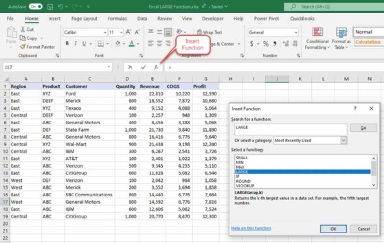
You can also type the function in the cell where you want to use it. Write "=LARGE(array, k)" in the cell, substituting your list of numeric values for "array." Instead of writing "k," put the rank of the numeric value you would like returned. To return the largest number, k should be the number one.
You can also add a helper column. Helper columns simplify complex formulas or difficult operations. You can use helper columns to sort and perform lookups with multiple criteria or in conjunction with formulas that return values for rows that meet specific conditions.
In this instance, the helper column is used to return the largest value.
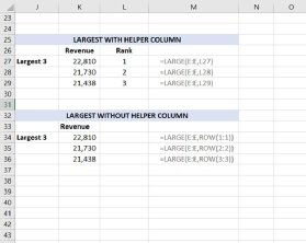
To set up the formulas, you should first build a helper column with the numbers 1, 2 and 3, as shown in L27:L29 in Figure 2.
In K27, write "=LARGE($E$2:$E$19,L27)." Doing so will return the largest value from E2:E19, which the MAX function can also produce. However, when you copy and paste the formula from K27 to K28 and K29, the formula will return the second-largest and third-largest values from the range.
However, you don't need to work with a helper column.
Each subsequent LARGE formula requires a higher value for the k argument. If you want the k argument to automatically increase as you copy down, use ROW(1:1) in the first formula. Now 1:1 is a reference to row 1. The ROW(1:1) is 1. The reference will change to 2:2 as you copy the formula down. Doing so returns the second-largest value and so on.
How to use the LARGE function in Excel
The main purpose of the LARGE function is to find a particular rank in a list. Being able to do so is especially useful if you want to find the top three or top five numbers in a list.
For example, you may need to find your company's top three revenue amounts.
Common LARGE function errors
The LARGE function is fairly straightforward to use, but some mistakes can happen. They include the following:
- You must include all the cells you want Excel to evaluate when you select a range of cells. For example, if the data includes 100 rows of data in a column, you must include all 100 rows when specifying the array to be evaluated. Doing so is an especially important consideration when you add additional data below the current array. If you add 10 rows of data to the existing list, you must update the array of cells in the LARGE function to include all 110 rows.
- You must also make sure the value of k is not too large for the data set. For example, if you have 10 rows of data and you set k to equal 11, you will get an error, since there are only 10 values.
- The LARGE function will evaluate numeric values, so the array should only contain numbers.
Example use cases
Use the LARGE function when you want to build a "top X" list of numbers based on the available data. For example, you may want to provide your sales department with employee performance data. You can use the LARGE function to display the top five sales amounts.
Another potential use case is an HR staff member gathering data on employee performance on a cybersecurity quiz. They can use the LARGE function to find the top five scores.
Related functions
Excel offers many other functions you can use to analyze data, including the SUM, MIN, MAX, SMALL and AVERAGE functions. The SUM() function, which adds a column of numbers, and the AVERAGE() function, which finds the average of a column of numbers, are among the most commonly used Excel functions. These functions only require one argument, which in this case is the range of cells you want to analyze.
For example, you can use the AutoSum icon or the Insert Function feature to enter =SUM(E2:E19) or =AVERAGE(E2:E19). You can only use AutoSum if the highlighted cells are in a contiguous row or column.
Finding the smallest numeric value in a column is more difficult, however, particularly if the cells aren't in a contiguous row or column.
You can use =MAX() and =MIN() to find the largest and smallest values in the range, respectively. Create the desired range by putting the cell numbers in the parentheses.
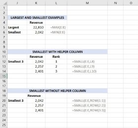
Figure 3 demonstrates how to find the largest and smallest values in Figure 1's Revenue column using =MAX() and =MIN(). The argument used for =MAX() and =MIN() is E2:E19, or simply select the whole column by writing (E:E) so the functions will return the top and bottom numbers from the Revenue column.
Use the =SMALL(array,k) function to return the smallest, second-smallest and third-smallest values from the range. Doing so is similar to the procedure for the LARGE function.
First, build a helper column with the numbers 1, 2 and 3, as shown in L12:L14 in Figure 3. In this instance, you are using the helper column to return the smallest value.
In K12, use =SMALL($E$2:$E$19,K12). Doing so returns the smallest value from E2:E19 and returns the identical result as using the MIN function. However, when you copy the formula from K12 to K13 and K14, the formula will return the second-smallest and third-smallest values from the range.
Avoiding the helper column
Similar to the LARGE function, you can avoid having to create a helper column by using the ROW function. To find the smallest number, put ROW(1:1) for the value of k.
Using pivot tables
If you'd like to avoid using formulas altogether, use a pivot table -- a reporting engine built into Excel that analyzes data without using formulas. Creating a pivot table is a relatively quick and simple process, especially if your source data is well-structured. When creating a pivot table, use good source data that is organized in a tabular layout. Doing so helps prevent future problems and will simplify the creation and maintenance of the pivot table.
To create one, first click on the Insert tab, then click on the PivotTable button. When the Create PivotTable dialog box appears, select the data you wish to use, then click OK. Drag a "label" field into the Row Labels area, then drag a numeric field into the Values area. Once you've created the table, you can program it to display data in your preferred order.
While LARGE and SMALL aren't the most popular functions, they're useful for finding the top three, top five, top 10 or bottom three values from a range.